Negative Values in A* Heuristics
Give an example of a graph - including nodes, links, link costs, and link cost estimates (heuristics) - that shows how allowing heuristics to take on negative values can temporarily mislead A*. Draw the graph and explain why A* generates more nodes for this graph than it would if you changed the negative h(.) values to 0.
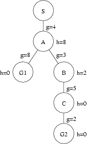
- Expanding S gives nodes A and B with f(A) = g(A) + h(A) = 3 + 1 = 4 and f(B) = g(B) + h(B) = 6 + -5 = 1. Since B has the lower value for f(.), it is placed before A in the open list and expanded first.
- Expanding B gives G2 with f(G2) = g(G2) + h(G2) = 8 + 0 = 8. Because G2 has a higher f(.) cost than A, it is placed behind A on the open list.
- Expanding A gives G1 with f(G1) = g(G1) + h(G1) = 5 + 0 = 5. Because G1 has a lower f(.) cost than G2, it is placed in front of G2 on the open list.
- G1 is removed from the open list and found to be a goal node - the search is finished.
- Expanding S gives nodes A and B with f(A) = g(A) + h(A) = 3 + 1 = 4 and f(B) = g(B) + h(B) = 6 + 0 = 6. Since A has the lower value for f(.), it is placed before B in the open list and expanded first.
- Expanding B gives G2 with f(G2) = g(G2) + h(G2) = 8 + 0 = 8. Because G2 has a higher f(.) cost than A, it is placed behind A on the open list. [Not done.]
- Expanding A gives G1 with f(G1) = g(G1) + h(G1) = 5 + 0 = 5. Because G1 has a lower f(.) cost than B, it is placed in front of B on the open list.
- G1 is removed from the open list and found to be the goal node - the search is finished.
Is A* still complete for graphs with negative h(.) values? Explain your answer.
Is A* still optimally efficient for graphs with negative h(.) values? Explain your answer.
- Expanding S gives nodes A and B with f(A) = g(A) + h(A) = 3 + 1 = 4 and f(B) = g(B) + h(B) = 6 + -5 = 1. Since B has the lower value for f(.), it is placed before A in the open list and expanded first.
- Expanding B gives G2 with f(G2) = g(G2) + h(G2) = 8 + -5 = 3. Because G2 has a lower f(.) cost than A, it is placed in front of A on the open list.
- Expanding A gives G1 with f(G1) = g(G1) + h(G1) = 5 + 0 = 5. Because G1 has a lower f(.) cost than G2, it is placed in front of G2 on the open list. [Not done.]
- G2 is removed from the open list and found to be a goal node - the search is finished.
Given two heuristics, (1) h(n) with some negative values and (2) h'(n) = MAX(h(n),0), does either heuristic dominate the other? Explain your answer.
Consider the following figure:
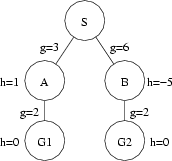
In this figure, S is the start node, G1 and G2 are both goal nodes, and A and B are intermediate nodes.
Repeating this example with the negative value for h(B) replaced with 0 proceeds as follows:
What we have observed is that repeating the example with 0 instead of -5 as the value for h(B) never generates node G2, i.e., the search is shorter. The search is shorter because without the negative value for h(B), the search was never mislead into thinking the route through B was likely to be shorter than the route through A.
(Note that negative h(.) values are not the only h(.) values that can be misleading. Consider the following figure:
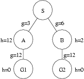
The order of node expansion and generation is exactly the same with this figure as it is with the figure above with a negative h(.) value. Moreover, if the h(.) value for node B were a more accurate estimate (say, 12), then the order of node expansion and generation for this figure would be exactly the same as with the figure above with the negative h(.) value replaced by 0.
In both cases, A* was mislead by poor h(.) values. The important difference with negative heuristic estimates is that we can rule out the possibility of negative path costs for a great many problems. For these problems, then, we know that the negative path cost estimates are poor estimates and can easily replace them with 0 (or whatever the minimum path cost might be), thereby improving the performance of our search algorithms in many cases.
On the other hand, for most problem domains we cannot easily tell when any given positive h(.) value is an underestimate and replace it with a better estimate. If we could, we'd simply use a better heuristic estimator to start with.)
No. Consider the following figure:
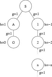
In this figure there is a goal node that is relatively close to the start node. It would be found quite quickly by complete search algorithms such as breadth-first search, uniform-cost search, and iterative-deepening depth-first search. However, the negative h(.) values in the right-hand branch of this tree would convince A* search to expand nodes in this branch forever, without ever considering the left-hand branch where the goal node is found. This is because for the right-hand branch, f(n) = g(n) + h(n) = n + -n = 0 for all n, whereas in the left-hand f(A) = g(A) + h(A) = 1 + 1 = 2. Since 0 is always more appealing than 2, A* will be fooled into following the wrong branch. This is another good reason why we don't allow negative h(.) values when using A*. (Thought of another way, this is why we should have A* change negative values to 0, if our heuristic function returns negative values.)
No. Consider the following figure:
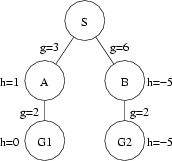
This figure is the same as the first figure given above, with the exception that there is a negative h(.) value for a goal node. The search will proceed as with the first example, except as indicated below (by highlighting/lowlighting).
Yes. The definition of dominates is that h2(n) dominates h1(n) iff "for any node n, h2(n) ≥ h1(n)" (p. 106). This is clearly the case here. MAX(h(n),0) ≥ h(n) (regardless of whether h(n) has some negative values).
PATHMAX in A* Search
Give an example of a graph - including nodes, links, link costs, and link cost estimates (heuristics) - that, when searched using A* with f(n) = g(n) + h(n) generates more nodes than when that same graph is searched using A* with PATHMAX. Draw the graph and explain why A* with f(n) = g(n) + h(n) generates more nodes than A* with PATHMAX.
- Expanding S gives node A with f(A) = g(A) + h(A) = 4 + 8 = 12. Since A is the only node generated, it is expanded.
- Expanding A gives G1 with f(G1) = g(G1) + h(G1) = 12 + 0 = 12 and B with f(B) = g(B) + h(B) = 7 + 2 = 9. Because G1 has a higher f(.) cost than B, it is placed behind B on the open list.
- Expanding B gives C with f(C) = g(C) + h(C) = 12 + 0 = 12. Because C has the same f(.) cost as G1 and is farther towards the front of the alphabet, it is placed behind G1 on the open list.
- G1 is removed from the open list and found to be a goal node - the search is finished.
- Expanding S gives node A with f(A) = g(A) + h(A) = 4 + 8 = 12. Since A is the only node generated, it is expanded.
- Expanding A gives G1 with f(G1) = MAX(g(G1)+h(G1), f(A)) = MAX(12+0,12) = 12 and B with f(B) = MAX(g(B)+h(B), f(A)) = MAX(7+2,12) = 12. Because G1 has the same f(.) cost as B and is farther towards the rear of the alphabet, it is placed in front of B on the open list.
- Expanding B gives C with f(C) = g(C) + h(C) = 12 + 0 = 12. Because C has the same f(.) cost as G1 and is farther towards the front of the alphabet, it is placed behind G1 on the open list. [Not done.]
- G1 is removed from the open list and found to be a goal node - the search is finished.
Is the heuristic you used in the previous part admissible? Explain your answer.
Is A* without PATHMAX optimally efficient with the heuristic you used in the previous part of this question? Explain your answer.
- Expanding S gives node A with f(A) = g(A) + h(A) = 4 + 8 = 12. Since A is the only node generated, it is expanded.
- Expanding A gives G1 with f(G1) = g(G1) + h(G1) = 12 + 0 = 12 and B with f(B) = g(B) + h(B) = 7 + 2 = 9. Because G1 has a higher f(.) cost than B, it is placed behind B on the open list.
- Expanding B gives C with f(C) = g(C) + h(C) = 12 + 0 = 12. Because C has the same f(.) cost as G1 and is farther towards the front of the alphabet, it is placed in front of G1 on the open list.
- Expanding C gives G2 with f(G2) = g(G2) + h(G2) = 14 + 0 = 14. Because G2 has a higher f(.) cost than G1, it is placed behind G1 on the open list.
- G1 is removed from the open list and found to be a goal node - the search is finished.
- Expanding S gives node A with f(A) = g(A) + h(A) = 4 + 8 = 12. Since A is the only node generated, it is expanded.
- Expanding A gives G1 with f(G1) = MAX(g(G1)+h(G1), f(A)) = MAX(12+0,12) = 12 and B with f(B) = MAX(g(B)+h(B), f(A)) = MAX(7+2,12) = 12. Because G1 has the same f(.) cost as B and is farther towards the rear of the alphabet, it is placed behind B on the open list.
- Expanding B gives C with f(C) = g(C) + h(C) = 12 + 0 = 12. Because C has the same f(.) cost as G1 and is farther towards the front of the alphabet, it is placed in front of G1 on the open list.
- Expanding C gives G2 with f(G2) = g(G2) + h(G2) = 14 +0 = 14. Because G2 has a higher f(.) cost than G1, it is placed behind G1 on the open list.
- G1 is removed from the open list and found to be a goal node - the search is finished.
At what point does PATHMAX allow us to discard nodes that we would otherwise explore using A*? Explain your answer.
Consider the following figure:
Assume that, given two nodes with equal f(.) values, A* will place the node with the letter that occurs farther towards the front of the alphabet farther towards the rear of the open list.
A* without PATHMAX searches this space as follows:
Compare this with the same search using PATHMAX:
Clearly, using PATHMAX we generated fewer nodes than we did without it. This is because PATHMAX raised the f(.) value for node B and, therefore, caused the nodes to be placed into the open list in a different order. Note, however, that this was only because of the "tie-breaking" criterion that put G1 in front of B when they had the same node values. If this criterion had been reversed (that is, if the node with the letter that occurs farther towards the front of the alphabet were to be placed farther towards the front of the open list), the placement of these two nodes in the open list would have been the same both with and without PATHMAX: B would have been placed before G1.
This is a little disappointing if we were under the impression that using PATHMAX would greatly help our search. However, this is the best PATHMAX can do: It can turn misleadingly low heuristic values into more accurate estimates but only to the extent that the poor estimates involved are now tied with the good estimates found elsewhere. It cannot guide us away from those nodes because it is only bringing up the estimates to an equal level - one coming from better estimates from ancestor nodes. Further, given that we have explored those ancestor nodes, we know that our path cost must be at least as expensive as the total path cost f(.) estimated at those ancestor nodes - the best path cost won't be lower than the f(.) estimates we are assigning using PATHMAX.
Yes. It is never overestimating, which is the definition of an admissible heuristic (p. 97). (I thought it was important to do this example solution using an admissible heuristic because, without one, we are not justified in using PATHMAX (or A*, for that matter). We only know that the estimate for h(B) is too low for this example if we know that h(A) is not too high.)
Yes. Because the heuristic used was admissible, A* is optimally efficient.
First, A* without PATHMAX is optimal. This is because it will keep pulling nodes off the open list and checking them to see if they are goal nodes until it finds one. When it finds one, all goal nodes not yet found must have a path cost at least as large as the path cost of the goal node found, assuming that the heuristic is admissible (as was the one in our example).
(Note that PATHMAX does not change this behavior of A*. As we have discussed above, PATHMAX can increase the costs assigned to nodes as they are generated but those new estimated path costs will not be overestimates. This is because we know that the cost being passed down from the parent is not an overestimate to begin with.)
Second, A* without PATHMAX is optimally efficient. For "algorithms that extend search paths from the root ... no other optimal algorithm is guaranteed to expand fewer nodes" than A* without PATHMAX, which is the definition of optimally efficient (p. 101).
As discussed in class and in the text, you can come up with examples in which some other optimal algorithm will happen to expand fewer nodes than an optimally efficient algorithm, due to tie-breakers. This is what we see in the example given here. To see why, imagine reversing the tie-breaker.
A* without PATHMAX searches this space as follows:
Compare this with the same search using PATHMAX:
What we see here is that, using a different tie-breaker, A* without PATHMAX expands no more nodes than A* with PATHMAX. The difference, in this case, was due solely to the tie-breaker used.
In fact, the difference between A* without PATHMAX and A* with PATHMAX will always come down to the tie-breaker used. This is because, as discussed above, all that PATHMAX can do is create ties where no ties existed before. It does this by setting a node's f(.) value equal to (not greater than) the f(.) value of it's ancestor(s). These new ties may be ordered in the open list by the tie-breaker in a different way for A* with PATHMAX than they were ordered in the open list by their (inaccurate) heuristic values using A* without PATHMAX, or they may be ordered in the open list in the same way in both cases.
However, what will not happen is that nodes that were stuck back farther in the open list due to higher f(.) values will be brought ahead of any of these nodes. This is because the new ties will not have f(.) values higher than the ancestor from which they are inheriting their new f(.) values and that ancestor was taken off the front of the open list because its f(.) value was less than or equal to the f(.) values of all the other nodes in the list. In other words, the tie-breaker will still decide the order of the nodes in play.
So, we can conclude that A* without PATHMAX is optimally efficient.
(On the other hand, this discussion of optimally efficient should make us think about whether being optimally efficient is the be all and end all of efficiency. After all, with the tie-breaker set one way, A* without PATHMAX generated more nodes than A* with PATHMAX; whereas with the tie-breaker set the other way, A* without PATHMAX generated the same number of nodes as A* with PATHMAX, but not fewer.
The general rule we see in this example has to do with dominating heuristics. Because A* with PATHMAX will effectively dominate A* without PATHMAX, A* with PATHMAX cannot expand more nodes than A* without PATHMAX, except possibly for some tie-breaking cases (from the discussion of domination on p. 106). However, since the only difference we have is in f(.) values, not the tie-breaker, A* with PATHMAX cannot expand more nodes than A* without PATHMAX.
On the contrary, A* with PATHMAX will sometimes generate fewer nodes than A* without PATHMAX. Those cases do depend on tie-breakers happening to work out in favor of A* with PATHMAX but their existence shows that A* with PATHMAX is sometimes better than A* without PATHMAX.
So, A* with PATHMAX is never worse, and sometimes better, than A* without PATHMAX. Yet, A* without PATHMAX is optimally efficient. This shouldn't concern or confuse us. It should, however, make us realize that dominating heuristics are a good thing from the standpoint of efficiency and what PATHMAX does is effectively create a new heuristic that dominates the original one, assuming the original one is non-monotonic.)
PATHMAX only allows us to discard nodes that we would otherwise explore using A* when we have taken a node off the open list and found it to be a goal node. Because A* with PATHMAX is complete, it must keep all nodes until it has found a goal node. Throwing away a node before finding a goal runs the risk of throwing away the last goal node (or a node on the last path to the goal node) and making the algorithm incomplete. Checking nodes to see if nodes are goals before throwing them away does not help because it would still be possible to throw away a node on the last path. PATHMAX does not, therefore, help with space requirements for open list storage. It may help, however, with storage space for the search tree being built and time spent generating and expanding nodes. (The downside is that the PATHMAX equation itself takes some time to run. This is true even when PATHMAX gives no benefits in space and time savings because the open list does not happen to be ordered any better with it than without it.)
Heuristic Domination
Give an example of a graph - including nodes, links, link costs, and two sets of link cost estimates h(.) and h'(.) such that h'(.) dominates h(.) - that, when searched using A* generates more nodes when using h'(.) than it does using h(.). Draw the graph and explain why A* generates more nodes with h'(.) than it does with h(.), even though h'(.) dominates.
- Expanding S gives nodes C and B with f(C) = g(C) + h(C) = 6 + 2 = 8 and f(B) = g(B) + h(B) = 6 + 1 = 7. Since B has the lower value for f(.), it is placed before C in the open list and expanded first.
- Expanding B gives G2 with f(G2) = g(G2) + h(G2) = 8 + 0 = 8. Because G2 has the same f(.) cost as C but is found later in the alphabet, it is placed in front of C on the open list.
- G2 is removed from the open list and found to be a goal node - the search is finished.
- Expanding S gives nodes C and B with f(C) = g(C) + h'(C) = 6 + 2 = 8 and f(B) = g(B) + h'(B) = 6 + 2 = 8. Since C has the same f(.) value as B but is found later in the alphabet, it is placed before B in the open list and expanded first.
- Expanding C gives G1 with f(G1) = g(G1) + h'(G1) = 11 + 0 = 11. Because G1 has a higher f(.) cost than B, it is placed behind B on the open list.
- Expanding B gives G2 with f(G2) = g(G2) + h'(G2) = 8 + 0 = 8. Because G2 has a lower f(.) cost than G1, it is placed in front of G1 on the open list.
- G2 is removed from the open list and found to be a goal node - the search is finished.
Explain why we prefer dominating heuristics in general.
Consider the following figure (and assume we are using the same tie-breaker as in Question 2.1):
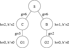
Using h(.) for our heuristic gives the following results:
Using h'(.) for our heuristic gives the following results:
As can be clearly seen from this example, A* using h'(.) generates (and expands) more nodes than A* using h(.), despite the fact that h'(.) dominates h(.). This is because, while h'(B) is a more accurate estimate of the remaining path cost from B to a goal node than is h(B), h(B) causes A* to try the better node first whereas h'(B) makes the path through B look no better to A* than the path through A, despite the fact that the path through B really is better. This is a case of the less accurate estimate leading the search in the correct direction fortuitously.
Note that, while h(B) helped to lead A* down the right path, h'(.) did not mislead A* down the wrong path. Instead, the choice between the right path and the wrong path came down to the tie-breaking criterion. If it had been reversed, A* with h'(.) would have chosen the right path first. This is another example of how a dominating heuristic can only be bested by the heuristic that it dominates due to tie-breakers, not by virtue of the values returned by the heuristics themselves.
(We could, of course, come up with a scenario in which h'(.) really did lead A* down the wrong path. Consider changing the values of h(C) and h'(C) to 1.5, for instance. In this case, A* using h'(.) will put C before B on the open list due to the lower f(.) value of C, rather than due to the tie-breaker. However, if we mislead A* with h'(.) we will also mislead A* with h(.). With the estimates of C changed to 1.5 in this example, A* with h(.) will no longer put G2 in front of C on the open list, since C will have a lower f(.) value. I.e., A* will be mislead into thinking C is on the better path using both h(.) and h'(.) and will expand it before checking to see if G2 is a goal node. Because h'(.) dominates h(.), any time h'(.) is deceptively inviting, h(.) will be as well.)
We prefer dominating heuristics in general, even though they can generate more nodes due to tie-breakers, because they are expected to generate fewer nodes more often than they generate more. This is because generating more nodes due to tie-breakers is happenstance. We would expect tie-breakers to work in our favor as often as they work against us. On the other hand, more accurate heuristic values should never mislead us on their own and should sometimes lead us in the correct direction on their own. The idea of heuristic values guiding our search so that we generate fewer nodes on the average is the whole reason we are using "informed" search methods.