CMPSCI/NSB 691C:
Homework #1: Population Codes

Andrew H. Fagg

This assignment focuses on the population code interpretation of neural activity. It is a pen-and-paper exercise and should require at most 2 hours to complete (including writing time). It is due at 5 pm on Tuesday, October 2nd.

Preferred Directions in Cartesian and Joint Space

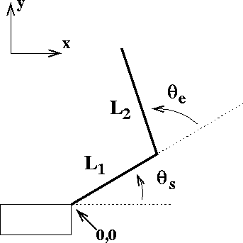
Figure 1 depicts a two-joint robot (or monkey) arm. The forward kinematics define the relationship between the arm's position in joint space ( $\theta = \left[{\theta_s \atop \theta_e}\right]$) and the endpoint of the arm ( $X = \left[{x \atop y}\right]$). Specifically:

$$L_1 \cos \theta_s + L_2 \cos(\theta_s + \theta_e)$$ x =

$$L_1 \sin \theta_s + L_2 \sin(\theta_s + \theta_e) .$$ y =

The Jacobian, $J(\theta)$ describes the local linear transformation from joint velocities to Cartesian velocities:

$$\dot{X} J(\theta)\dot{\theta}$$ =

$$\left[ \begin{array}{cc} \frac{\partial x}{\partial \theta_s} & \... ...eft[ \begin{array}{c} \dot{\theta_s} \\ \\ \dot{\theta_e} \end{array}\right],$$ =

where:

$$\frac{\partial x}{\partial \theta_s} -L_1 \sin \theta_s - L_2 \sin(\theta_s+\theta_e)$$ =

$$\frac{\partial x}{\partial \theta_e} - L_2 \sin(\theta_s+\theta_e)$$ =

$$\frac{\partial y}{\partial \theta_s} L_1 \cos \theta_s + L_2 \cos(\theta_s+\theta_e)$$ =

$$\frac{\partial y}{\partial \theta_e} L_2 \cos(\theta_s+\theta_e).$$ =

  

Figure: Kinematic model of a two-link arm. $\theta_s$ and $\theta_e$ are the joint angles for the shoulder and elbow, respectively. L₁ and L₂ are the link lengths. The origin of the Cartesian coordinate system is rooted at the shoulder.

We will assume that L₁ = L₂ = 1 and that a movement from a starting point to a target is very small. The latter allows us to assume that a movement can be expressed as an instantaneous velocity (i.e. as $\dot{X}$ and $\dot{\theta}$).

Suppose that a cell in MI has a ``real'' preferred direction in joint space of $\dot{\theta} = \left[ {1 \atop -1} \right]$.

Question 1.1: At position $\theta = \left[ {\frac{\pi}{4} \atop \frac{\pi}{2}} \right]$, what is the apparent preferred direction in Cartesian space?

Answer: $\dot{X} = \left[ {-\frac{\sqrt{2}}{2} \atop \frac{\sqrt{2}}{2}} \right]$

Question 1.2: At position $\theta = \left[ {0 \atop \frac{\pi}{2}} \right]$, what is the cell's apparent preferred direction?

Answer: $\dot{X} = \left[ {0 \atop 1} \right]$

Suppose an MI cell has a ``real'' preferred direction of $\dot{X} = \left[ {1 \atop 0} \right]$.

Question 1.3: At position $\theta = \left[ {\frac{\pi}{4} \atop \frac{\pi}{2}} \right]$, what is the apparent preferred direction in joint space?

Answer: $\dot{\theta} = \left[ {-\frac{1}{\sqrt{2}} \atop 0} \right]$

Question 1.4: At position $\theta = \left[ {0 \atop \frac{\pi}{2}} \right]$, what is the cell's apparent preferred direction in joint space?

Answer: $\dot{\theta} = \left[ {0 \atop -1} \right]$

The model for cell discharge used by Georgopolous et al. was:

$$d(\psi) = a + b \cos\left(\psi - \psi_{pref}\right),$$ (1)

where $d(\psi)$ is the cell discharge rate, $\psi$ is the direction of movement in Cartesian space and a, b, and $\psi_{pref}$ are parameters.

Question 1.5: Construct an equivalent model for a cell that encodes movement in joint coordinates. In other words, give an expression for the cell discharge rate as a function of $\dot{\theta}_e$ and $\dot{\theta}_s$. Note that there is not a unique answer.

$$d(\dot{\theta}) a + b \cos\left(atan2(\dot{\theta_e}, \dot{\theta_s}) - \psi_{pref}\right)$$ = (2)

Georgopolous' ``cosine tuning function'' is but one way to describe the transformation of a distance metric (in this case $\theta_{movement} - \theta_{pref}$) into a cell discharge rate. It happens to be very convenient because relative orientation and the cosine function are both periodic in nature. But - it does not have to be this way...

Suppose that instead of coding movement direction, we would like to encode a description of object shape and size (e.g., as extracted by the visual system). The shapes and parameters that we would like our population of cells to encode are:

Shape	Parameters
sphere	diameter
cylinder	diameter, length
box	length, width, height

Question 1.6: Give one possible population coding scheme for this set of objects. In other words, for the set of cells, write an expression (or expressions) representing the cells' discharge rate as a function of the exact object being coded.

One Answer: Assume that there are three separate populations of neurons - one for each of the different shapes. For any particular shape, only those cells that encode that shape will be active.

For sphere cells:

d_i^s(diam) = a_i + b_i G_i(diam - diam_pref,i).

For cylinder cells:

d_i^c(diam, len) = a_i + b_i G_i(diam - diam_pref,i) + c_i G_i(len - len_pref,i) .

For box cells:

d_i^b(len, width, height) = a_i + b_i G_i(len - len_pref,i) + c_i G_i(width - width_pref,i) + f_i G_i(height - height_pref,i) .

Where G_i() is Gaussian in shape:

$$e^{-\left(\frac{x}{\sigma_i}\right)^2}$$ G_i(x) =

Another Answer: same as above, but with multidimensional Gaussians.

For sphere cells:

d_i^s(diam) = a_i + b_i G_i(diam - diam_pref,i).

For cylinder cells:

$$a_i + b_i G_i \left( \left [ {diam - diam_{pref,i}} \atop {len - len_{pref,i}} \right ] \right ).$$ d_i^c(diam, len) =

For box cells:

$$a_i + b_i G_i\left( \left[ \begin{array}{c} {len - len_{pref,i}} ... ... - width_{pref,i}} \\ {height - height_{pref,i}} \end{array}\right ] \right) .$$ d_i^b(len, width, height) =

Where G_i() is Gaussian in shape:

$$e^{-\left(\mathbf{x}^T\; \mathbf{M_i}\; \mathbf{x}\right)},$$ G_i(x) =

and where M_i is a scaling matrix.

About this document ...

CMPSCI/NSB 691C:
Homework #1: Population Codes

This document was generated using the LaTeX2HTML translator Version 98.1p1 release (March 2nd, 1998)

Copyright © 1993, 1994, 1995, 1996, 1997, Nikos Drakos, Computer Based Learning Unit, University of Leeds.

The command line arguments were:
latex2html -no_navigation -split 0 -t CMPSCI/NSB 691C: HW1 -dir html -no_reuse -tmp /tmp hw1.tex.

The translation was initiated by Andrew H. Fagg on 2001-10-04