CS 5043: HW8: Semantic Labeling
Assignment notes:
- Deadline:
- Deadline: Friday, May 6th @11:59pm.
- Hand-in procedure: submit a zip file to Gradescope
- This work is to be done on your own. While general discussion
about Python, Keras and Tensorflow is encouraged, sharing
solution-specific code is inappropriate. Likewise, downloading
solution-specific code is not allowed.
- Do not submit MSWord documents.
Data Set
The Chesapeake Watershed data set is derived from satellite imagery
over all of the US states that are part of the Chesapeake Bay
watershed system. We are using the patches part of the data
set. Each patch is a 256 x 256 image with 26 channels, in which each
pixel corresponds to a 1m x 1m area of space. Some of these
channels are visible light channels (RGB), while others encode surface
reflectivity at different frequencies. In addition, each pixel is
labeled as being one of:
- 0 = no class
- 1 = water
- 2 = tree canopy / forest
- 3 = low vegetation / field
- 4 = barren land
- 5 = impervious (other)
- 6 = impervious (road)
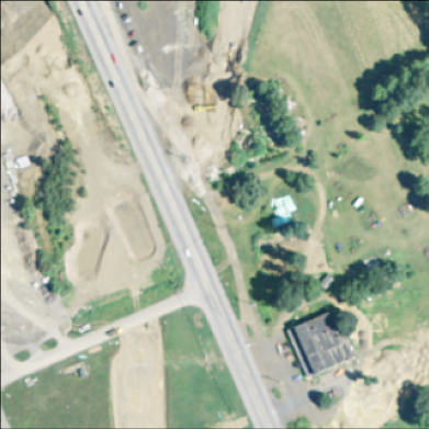
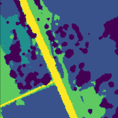
Here is an example of the RGB image of one patch and the corresponding pixel labels:
Notes:
Data Organization
All of the data are located on the supercomputer in:
/home/fagg/datasets/radiant_earth/pa. Within this directory, there are both
train and valid directories. Each of these contain
directories F0 ... F9 (folds 0 to 9). Each training fold is composed
of 5000 patches. Because of the size of the folds, we have provided
code that produces a TF Dataset that dynamically loads the data as you
need it. We will use the train directory to draw our training
and validation sets from and the valid directory to draw our
testing set from.
Local testing: the file chesapeake_small.zip
contains the data for folds 0 and 9 (it is 6GB compressed).
Within each fold directory, the files are of the form:
SOME_NON_UNIQUE_HEADER-YYY.npz. Where YYY is 0 ... 499 (all
possible YYYs occur in each fold directory. There are multiple files
with each YYY number in each directory (100 in the training fold
directories, to be precise).
Data Access
chesapeake_loader.py is provided. The key function call is:
dataset = create_dataset(base_dir='/home/fagg/datasets/radiant_earth/pa',
                         partition='train', fold=0, filt='*',
                         batch_size=8, prefetch=2, num_parallel_calls=4):
where:
- dataset is a TF Dataset object that loads and manages
your data
- base_dir is the main directory for the dataset
- partition is the subdirectory to use ("train" or
"valid")
- fold is the fold to load (0 ... 9)
- filt is a regular expression filter that specifies which
file numbers to include.
- '*0' will load all numbers ending with zero (500 examples).
- '*[01234]' will load all numbers ending with 0,1,2,3 or 4.
- '*' will load all 5000 examples.
- batch_size is the size of the batches produced by your
dataset
- prefetch is the number of batches that will be buffered
- num_parallel_calls is the number of threads to use to
create the Dataset
The returned Dataset will generate batches of the specified size of
input/output tuples.
- Inputs: floats: batch_size x 256 x 256 x 26
- Outputs: int8: batch_size x 256 x 256
A returned Dataset can be used for fitting or evaluating a model.
The Problem
Create an image-to-image translator that does semantic labeling of the
images.
Details:
- Your network output should be shape (examples, rows, cols,
class), where the sum of all class outputs for a single pixel
is 1 (i.e., we are using a softmax across the last dimension of
your output).
- Use tf.keras.losses.SparseCategoricalCrossentropy as
your loss function. This will properly translate between your
one-output per class per pixel to the outs that have
just one class label for each pixel.
- Use tf.keras.metrics.SparseCategoricalAccuracy as an
evaluation metric. Because of the class imbalance, a model
that predicts the majority class will have an accuracy of ~0.65
- Try using a sequential-style model, as well as a U-net model.
Deep Learning Experiment
For what you think is your best performing model type (and
hyper-parameters), perform 5 different experiments:
- Use '*[012345678]' for training (train partition). Note: when
debugging, just use '*0'
- Use '*[9]' for validation (train partition)
- Use '*' for testing (valid partition)
The five different experiments will use folds F0 ... F4 (so, no
overlap in any of the datasets).
Reporting
- Figure 1: model architecture from plot_model(). One figure
- Figure 2: Validation accuracy as a function of training epoch.
Show 5 curves.
- Figures 3...7: for each model, evaluate using the test data set
and generate a confusion matrix. (so, one confusion matrix per
rotation)
- Figure 8: histogram of test accuracy. Plot a vertical line
indicating the mean (and give the mean as text on the figure)
- Figure 9: for one model, show three examples (one per row).
Each row includes: Satellite image (channels 0,1,2); true
labels; predicted labels.
plt.imshow can be useful here, but make sure for the label
images that the label-to-color mapping is the same
What to Hand In
Hand in a PDF file that contains:
- All of your python code (.py) and any notebook file (.ipynb)
[Gradescope can render notebook files directly - no need to
convert to pdf!]
- Figures 1-9
Grades
- 20 pts: Clean, general code for model building (including
in-code documentation)
- 5 pts: Figure 1
- 10 pts: Figure 2
- 5 pts each: Figures 3-7
- 10 pts: Figure 8
- 10 pts: Figure 9
- 20 pts: Reasonable test set performance for all rotations
References
Hints
- Start small. Get the architecture working before throwing lots
of data at it.
- Write generic code.
- Start early. Expect the learning process for these models to
exceed anything else that we have done in the class.
andrewhfagg -- gmail.com
Last modified: Mon May 2 14:14:52 2022